Julia CFD｜09 二维扩散问题

二维扩散问题控制方程可写出下面形式：

这里时间项采用向前差分，空间项均采用中心差分，很容易写出离散方程：

同样写出待求项：

初始条件及边界条件见代码。

using PyPlot
 
nx = 101
ny = 101
nu = 0.2
dx = 2 / (nx - 1)
dy = 2 / (ny - 1)
sigma = 0.25
dt = sigma * dx * dy / nu
 
x = range(0, 2, length=nx)
y = range(0, 2, length=ny)
 
u = ones(ny, nx)
un = ones(ny, nx)
# 初始化
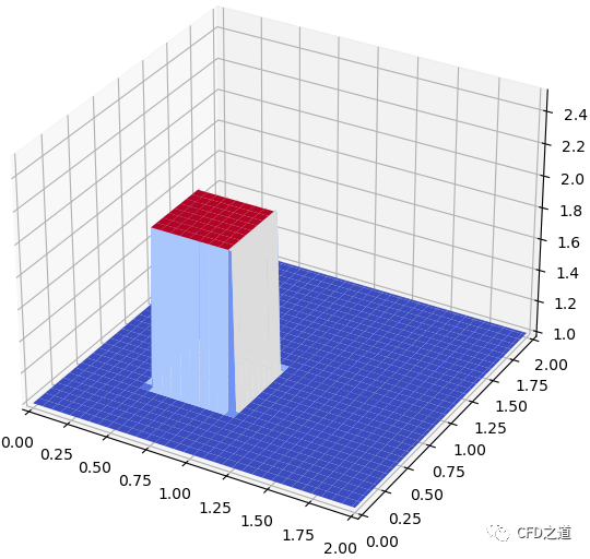
u[floor(Int, 0.5 / dy):floor(Int, 1 / dy),floor(Int, 0.5 / dx):floor(Int, 1 / dx)] .= 2
 
# 绘制初始值
PyPlot.surf(x,y,u)
xlim(0,2)
ylim(0,2)
zlim(1,2.5)
PyPlot.show()

初始条件如下图所示。

下面定义函数进行求解。

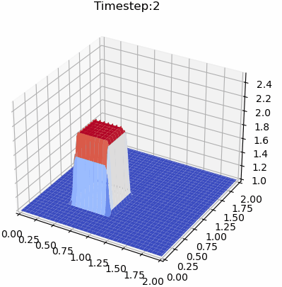
function diffuse(nt)
    for n in 1:nt
        PyPlot.cla()
        un = copy(u)
        u[2:end - 1,2:end - 1] = un[2:end - 1,2:end - 1] + nu * dt / dx^2 * (un[2:end - 1,3:end] - 2 * un[2:end - 1,2:end - 1] + un[2:end - 1,1:end - 2]) + nu * dt / dy^2 * (un[3:end,2:end - 1] - 2 * un[2:end - 1,2:end - 1] + un[1:end - 2,2:end - 1])
        u[1,:] .= 1
        u[end,:] .= 1
        u[:,1] .= 1
        u[1,end] = 1
    end
 
    PyPlot.surf(x, y, u, cmap=ColorMap("coolwarm"))
    PyPlot.xlim(0, 2)
    PyPlot.ylim(0, 2)
    PyPlot.zlim(1, 2.5)
    PyPlot.title(@sprintf("Timestep:%d",nt))   
    PyPlot.pause(.2)
    PyPlot.show()
end

下面进行计算。

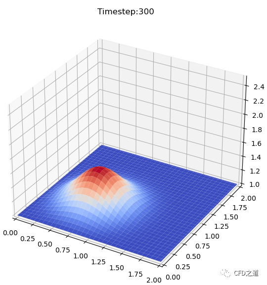
diffuse(300)

图形如下图所示。

改造成以下的完整代码以动画形式显示扩散过程。

using PyPlot
using Printf
 
nx = 101
ny = 101
nu = 0.2
dx = 2 / (nx - 1)
dy = 2 / (ny - 1)
sigma = 0.25
dt = sigma * dx * dy / nu
 
x = range(0, 2, length=nx)
y = range(0, 2, length=ny)
 
u = ones(ny, nx)
u[floor(Int, 0.5 / dy):floor(Int, 1 / dy),floor(Int, 0.5 / dx):floor(Int, 1 / dx)] .= 2
# 显示初始条件
# PyPlot.surf(x,y,u)
# xlim(0,2)
# ylim(0,2)
# zlim(1,2.5)
# PyPlot.show()
 
function diffuse(nt)
    for n in 1:nt
        PyPlot.cla()
        un = copy(u)
        u[2:end - 1,2:end - 1] = un[2:end - 1,2:end - 1] + nu * dt / dx^2 * (un[2:end - 1,3:end] - 2 * un[2:end - 1,2:end - 1] + un[2:end - 1,1:end - 2]) + nu * dt / dy^2 * (un[3:end,2:end - 1] - 2 * un[2:end - 1,2:end - 1] + un[1:end - 2,2:end - 1])
        u[1,:] .= 1
        u[end,:] .= 1
        u[:,1] .= 1
        u[1,end] = 1
 
        PyPlot.surf(x, y, u, cmap=ColorMap("coolwarm"))
        PyPlot.xlim(0, 2)
        PyPlot.ylim(0, 2)
        PyPlot.zlim(1, 2.5)
        PyPlot.title(@sprintf("Timestep:%d",n))   
        PyPlot.pause(.2)
    end
    PyPlot.show()
end
 
diffuse(300)

计算结果如下图所示。