接下来,我们将以Burgers方程作为强化学习(RL)的测试平台来针对反问题。该设置类似于之前使用可微物理(DP)训练针对的反问题(参见{doc}diffphys-code-control),因此我们将在下面直接进行比较。与之前类似,Burgers方程是简单但非线性的,具有有趣的动力学,因此是RL实验的一个良好起点。在接下来的过程中,目标是训练一个控制力估计网络,该网络应该预测生成两个给定状态之间平滑过渡所需的力。
16.1 概述
强化学习描述了一个代理在感知环境并在其中采取行动的过程。它旨在最大化代理通过环境采取的行动所获得的奖励累积和。因此,代理通过经验学习在不同情况下采取哪些行动。近端策略优化 (PPO)是一种广泛使用的强化学习算法,描述了两个神经网络:一个策略神经网络根据给定的观测选择行动,一个值估计网络评估这些状态的奖励潜力。这些值估计形成了策略网络的损失,即所选行动带来的奖励潜力变化。
本笔记本演示了如何将PPO强化学习应用于Burgers方程的控制问题。与DP方法相比,RL方法没有可微分的物理求解器,它是无模型的。然而,值估计神经网络的目标是弥补这种求解器的缺失,因为它试图捕捉单个行动的长期效应。因此,以下代码示例应该回答一个有趣的问题:无模型PPO强化学习能否匹配基于模型的DP训练的性能。我们将比较学习速度和所需力量的数量。
16.2 软件安装
本示例使用强化学习框架stable_baselines3,其中采用PPO作为强化学习算法。
对于物理仿真,使用可微分PDE求解器ΦFlow的1.5.1版本。在完成RL训练后,我们还将使用“控制力估计器”(CFE)网络从{doc}diffphys-code-control(由{cite}holl2019pdecontrol引入)引入可微分物理方法进行额外比较。
!pip install stable-baselines3==1.1 phiflow==1.5.1
!git clone https://github.com/Sh0cktr4p/PDE-Control-RL.git
!git clone https://github.com/holl-/PDE-Control.git
现在我们可以导入必要的模块。由于这个示例的范围比较大,需要加载相当多的模块。
import sys; sys.path.append('PDE-Control/src'); sys.path.append('PDE-Control-RL/src')
import time, csv, os, shutil
from tensorboard.backend.event_processing.event_accumulator import EventAccumulator
from phi.flow import *
import burgers_plots as bplt
import matplotlib.pyplot as plt
from envs.burgers_util import GaussianClash, GaussianForce
16.3 数据生成
首先,我们生成一个数据集用于训练可微分物理模型。我们还将使用它来在训练期间和训练后评估两种方法的性能。下面的代码模拟了1000个情况(即phiflow“场景”),并将其中的100个作为验证和测试用例。剩下的800个用于训练。
DOMAIN = Domain([32], box=box[0:1])     # Size and shape of the fields
VISCOSITY = 0.003
STEP_COUNT = 32                         # Trajectory length
DT = 0.03
DIFFUSION_SUBSTEPS = 1

DATA_PATH = 'forced-burgers-clash'
SCENE_COUNT = 1000
BATCH_SIZE = 100

TRAIN_RANGE = range(200, 1000)
VAL_RANGE = range(100, 200)
TEST_RANGE = range(0, 100)

for batch_index in range(SCENE_COUNT // BATCH_SIZE):
    scene = Scene.create(DATA_PATH, count=BATCH_SIZE)
    print(scene)
    world = World()
    u0 = BurgersVelocity(
        DOMAIN,
        velocity=GaussianClash(BATCH_SIZE),
        viscosity=VISCOSITY,
        batch_size=BATCH_SIZE,
        name='burgers'
    )
    u = world.add(u0, physics=Burgers(diffusion_substeps=DIFFUSION_SUBSTEPS))
    force = world.add(FieldEffect(GaussianForce(BATCH_SIZE), ['velocity']))
    scene.write(world.state, frame=0)
    for frame in range(1, STEP_COUNT + 1):
        world.step(dt=DT)
        scene.write(world.state, frame=frame)
输出:
forced-burgers-clash/sim_000000
forced-burgers-clash/sim_000100
forced-burgers-clash/sim_000200
forced-burgers-clash/sim_000300
forced-burgers-clash/sim_000400
forced-burgers-clash/sim_000500
forced-burgers-clash/sim_000600
forced-burgers-clash/sim_000700
forced-burgers-clash/sim_000800
forced-burgers-clash/sim_000900
16.4 通过强化学习进行训练
接下来我们建立强化学习环境。PPO方法使用一个专门的价值估计网络(“评论家”)来预测从某个状态产生的奖励总和。然后使用这些预测的奖励来更新策略网络(“演员”),类似于{doc}diffphys-code-control中的CFE网络,预测用于控制模拟的力。
from experiment import BurgersTraining

N_ENVS = 10                         # On how many environments to train in parallel, load balancing
FINAL_REWARD_FACTOR = STEP_COUNT    # Penalty for not reaching the goal state
STEPS_PER_ROLLOUT = STEP_COUNT * 10 # How many steps to collect per environment between agent updates
N_EPOCHS = 10                       # How many epochs to perform during each agent update
RL_LEARNING_RATE = 1e-4             # Learning rate for agent updates
RL_BATCH_SIZE = 128                 # Batch size for agent updates
RL_ROLLOUTS = 500                  # Number of iterations for RL training
为了开始训练,我们创建一个管理环境和代理的训练器对象。此外,还创建了一个用于存储模型、日志和超参数的目录。这样,可以使用相同的配置在任何后续时间继续训练。如果在exp_name中指定的模型文件夹已经存在,则加载其中的代理;否则,创建一个新的代理。对于PPO强化学习算法,使用stable_baselines3的实现。训练器类作为该系统的包装器。在底层,创建了一个BurgersEnv gym环境的实例,该环境加载到PPO算法中。它生成随机的初始状态,预计算相应的地面真实模拟,并处理受代理行动影响的系统演化。此外,训练器定期通过加载使用验证集的初始和目标状态的不同环境来评估性能。
16.5 Gym环境
Gym环境规范提供了利用代理交互的接口。实现它的环境必须指定观察和动作空间,它们表示代理策略的输入和输出空间。此外,它们还必须定义一组方法,其中最重要的有 reset、step 和 render。
reset在轨迹结束后被调用,以将环境重置为初始状态,并返回相应的观察结果。step获取代理给出的行动,并将环境迭代到下一个状态。它返回所得到的观察结果、收到的奖励、确定是否达到终端状态的标志以及用于调试和日志记录信息的字典。render被调用以以环境创建者指定的方式显示当前环境状态。此函数可用于检查训练结果。
与默认的 gym 环境相比,stable-baselines3 通过提供支持向量化环境的接口进行了扩展。这使得可以对多个轨迹同时计算前馈传播,从而由于更好的资源利用而增加时间效率。在实践中,这意味着这些方法现在在观测结果、行动、奖励、终端状态标志和信息字典的向量上运行。步骤方法分为 step_async 和 step_wait,使每个环境实例能够在不同线程上运行成为可能。
16.6 物理仿真
Burgers方程的环境包含由phiflow提供的Burgers物理对象。状态在内部存储为BurgersVelocity对象。为了创建初始状态,环境以与上面显示的数据集生成过程相同的方式生成一批随机字段。观测空间由叠加在通道维度中的当前状态和目标状态的速度场组成,另一个通道指定当前时间步长。动作以覆盖每个速度值的一维阵列的形式进行。step方法调用物理对象将内部状态提前一个时间步长,也将这些动作应用为FieldEffect。
奖励包括一个等于每个时间步长产生的力的平方范数的惩罚。此外,在每个轨迹的末尾减去按预定义因子(FINAL_REWARD_factor)缩放的到目标场的距离。然后用对奖励平均值和标准差的运行估计对奖励进行归一化。
16.7 神经网络设置
我们使用两种不同的神经网络架构分别用于演员和评论家。前者使用{cite}holl2019pdecontrol中的U-Net变体,而后者由一系列1D卷积和池化层组成,将特征映射大小降至1。最后的操作是使用核大小为1的卷积将特征映射组合并保留一个输出值。然后,CustomActorCriticPolicy类使得可以使用这两个独立的网络架构来进行强化学习代理。
默认情况下,代理存储在PDE-Control-RL/networks/rl-models/bench中,并在存在时加载。 (如果需要,将下面的path替换为新的路径以从新模型开始。)由于训练时间较长,因此我们在这里使用预先训练的代理。它已经训练了3500个迭代,因此我们只需通过另外的RL_ROLLOUTS=500迭代进行“微调”。这些通常需要大约2个小时,因此几乎18个小时的总训练时间对于交互式测试来说太长了。 (但是,如果您拥有资源,此处提供的代码包含从头开始训练模型的所有内容。)
rl_trainer = BurgersTraining(
    path='PDE-Control-RL/networks/rl-models/bench', # Replace path to train a new model
    domain=DOMAIN,
    viscosity=VISCOSITY,
    step_count=STEP_COUNT,
    dt=DT,
    diffusion_substeps=DIFFUSION_SUBSTEPS,
    n_envs=N_ENVS,
    final_reward_factor=FINAL_REWARD_FACTOR,
    steps_per_rollout=STEPS_PER_ROLLOUT,
    n_epochs=N_EPOCHS,
    learning_rate=RL_LEARNING_RATE,
    batch_size=RL_BATCH_SIZE,
    data_path=DATA_PATH,
    val_range=VAL_RANGE,
    test_range=TEST_RANGE,
)
Tensorboard log path: PDE-Control-RL/networks/rl-models/bench/tensorboard-log
Loading existing agent from PDE-Control-RL/networks/rl-models/bench/agent.zip
下面的单元格是可选的,但对于调试非常有用:它在笔记本内打开_tensorboard_以显示训练的进度。如果在不同位置创建了一个新模型,请相应地更改路径。当恢复预训练代理的学习过程时,新运行将在tensorboard中单独显示(通过齿轮按钮启用重新加载)。
名为“forces”的图表显示了网络生成的总力量随着训练的演变情况。“rew_unnormalized”显示了未进行上述归一化步骤的奖励值。对应的归一化值在“rollout/ep_rew_mean”下方显示。“val_set_forces”概述了代理在验证集上的表现。
%load_ext tensorboard
%tensorboard --logdir PDE-Control-RL/networks/rl-models/bench/tensorboard-log
现在我们已经准备好开始对代理进行训练了。强化学习方法需要进行多次迭代来探索环境。因此,下一个单元格通常需要多个小时才能执行完毕(500次模拟需要大约2小时)。
rl_trainer.train(n_rollouts=RL_ROLLOUTS, save_freq=50)
Storing agent and hyperparameters to disk...
Storing agent and hyperparameters to disk...
Storing agent and hyperparameters to disk...
Storing agent and hyperparameters to disk...
Storing agent and hyperparameters to disk...
Storing agent and hyperparameters to disk...
Storing agent and hyperparameters to disk...
Storing agent and hyperparameters to disk...
Storing agent and hyperparameters to disk...
Storing agent and hyperparameters to disk...
Storing agent and hyperparameters to disk...
Storing agent and hyperparameters to disk...
16.8 RL 评估
现在我们有了一个训练好的模型,让我们来看看结果。最左边的图显示了强化学习代理的结果。作为参考,在其旁边显示了地面真相,即代理应该重建的轨迹,以及未受控制的模拟,其中系统遵循其自然演化。
TEST_SAMPLE = 0    # Change this to display a reconstruction of another scene
rl_frames, gt_frames, unc_frames = rl_trainer.infer_test_set_frames()

fig, axs = plt.subplots(1, 3, figsize=(18.9, 9.6))
axs[0].set_title("Reinforcement Learning"); axs[1].set_title("Ground Truth"); axs[2].set_title("Uncontrolled")
for plot in axs:
    plot.set_ylim(-2, 2); plot.set_xlabel('x'); plot.set_ylabel('u(x)')

for frame in range(0, STEP_COUNT + 1):
    frame_color = bplt.gradient_color(frame, STEP_COUNT+1);
    axs[0].plot(rl_frames[frame][TEST_SAMPLE,:], color=frame_color, linewidth=0.8)
    axs[1].plot(gt_frames[frame][TEST_SAMPLE,:], color=frame_color, linewidth=0.8)
    axs[2].plot(unc_frames[frame][TEST_SAMPLE,:], color=frame_color, linewidth=0.8)
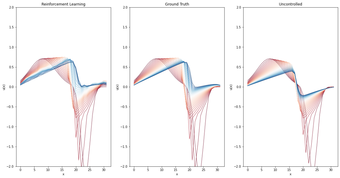
正如我们所看到的,经过训练的强化学习代理能够相当好地重构轨迹。然而,它们仍然显著比真实情况不够平滑。
16.9 可微物理训练
为了对强化学习方法的结果进行分类,我们现在将它们与可微分物理训练方法进行比较。与包括第二个_OP_网络的完整方法相比,我们在这里旨在直接控制。OP网络代表一个独立的“物理预测器”,在与RL版本进行比较时为公平起见,我们省略了它。
DP方法可以访问由可微分求解器提供的梯度数据,从而可以跟踪多个时间步长的损失,并使模型更好地理解所生成力的长期效应。另一方面,强化学习算法不像DP算法那样受训练集大小的限制,因为新的训练样本是在策略上生成的。然而,这也在训练期间引入了额外的模拟开销,可能会增加收敛所需的时间。
from control.pde.burgers import BurgersPDE
from control.control_training import ControlTraining
from control.sequences import StaggeredSequence
Could not load resample cuda libraries: CUDA binaries not found at /usr/local/lib/python3.7/dist-packages/phi/tf/cuda/build/resample.so. Run "python setup.py cuda" to compile them
下面的单元格设置用于训练模型或加载现有模型检查点。
dp_app = ControlTraining(
    STEP_COUNT,
    BurgersPDE(DOMAIN, VISCOSITY, DT),
    datapath=DATA_PATH,
    val_range=VAL_RANGE,
    train_range=TRAIN_RANGE,
    trace_to_channel=lambda trace: 'burgers_velocity',
    obs_loss_frames=[],
    trainable_networks=['CFE'],
    sequence_class=StaggeredSequence,
    batch_size=100,
    view_size=20,
    learning_rate=1e-3,
    learning_rate_half_life=1000,
    dt=DT
).prepare()
App created. Scene directory is /root/phi/model/control-training/sim_000000 (INFO), 2021-08-04 10:11:58,466n
Sequence class: <class 'control.sequences.StaggeredSequence'> (INFO), 2021-08-04 10:12:01,449n
Partition length 32 sequence (from 0 to 32) at frame 16
Partition length 16 sequence (from 0 to 16) at frame 8
Partition length 8 sequence (from 0 to 8) at frame 4
Partition length 4 sequence (from 0 to 4) at frame 2
Partition length 2 sequence (from 0 to 2) at frame 1
Execute -> 1
Execute -> 2
Partition length 2 sequence (from 2 to 4) at frame 3
Execute -> 3
Execute -> 4
Partition length 4 sequence (from 4 to 8) at frame 6
Partition length 2 sequence (from 4 to 6) at frame 5
Execute -> 5
Execute -> 6
Partition length 2 sequence (from 6 to 8) at frame 7
Execute -> 7
Execute -> 8
Partition length 8 sequence (from 8 to 16) at frame 12
Partition length 4 sequence (from 8 to 12) at frame 10
Partition length 2 sequence (from 8 to 10) at frame 9
Execute -> 9
Execute -> 10
Partition length 2 sequence (from 10 to 12) at frame 11
Execute -> 11
Execute -> 12
Partition length 4 sequence (from 12 to 16) at frame 14
Partition length 2 sequence (from 12 to 14) at frame 13
Execute -> 13
Execute -> 14
Partition length 2 sequence (from 14 to 16) at frame 15
Execute -> 15
Execute -> 16
Partition length 16 sequence (from 16 to 32) at frame 24
Partition length 8 sequence (from 16 to 24) at frame 20
Partition length 4 sequence (from 16 to 20) at frame 18
Partition length 2 sequence (from 16 to 18) at frame 17
Execute -> 17
Execute -> 18
Partition length 2 sequence (from 18 to 20) at frame 19
Execute -> 19
Execute -> 20
Partition length 4 sequence (from 20 to 24) at frame 22
Partition length 2 sequence (from 20 to 22) at frame 21
Execute -> 21
Execute -> 22
Partition length 2 sequence (from 22 to 24) at frame 23
Execute -> 23
Execute -> 24
Partition length 8 sequence (from 24 to 32) at frame 28
Partition length 4 sequence (from 24 to 28) at frame 26
Partition length 2 sequence (from 24 to 26) at frame 25
Execute -> 25
Execute -> 26
Partition length 2 sequence (from 26 to 28) at frame 27
Execute -> 27
Execute -> 28
Partition length 4 sequence (from 28 to 32) at frame 30
Partition length 2 sequence (from 28 to 30) at frame 29
Execute -> 29
Execute -> 30
Partition length 2 sequence (from 30 to 32) at frame 31
Execute -> 31
Execute -> 32
Target loss: Tensor("truediv_1:0", shape=(), dtype=float32) (INFO), 2021-08-04 10:13:10,701n

Force loss: Tensor("Sum_97:0", shape=(), dtype=float32) (INFO), 2021-08-04 10:13:14,221n

Setting up loss (INFO), 2021-08-04 10:13:14,223n

Preparing data (INFO), 2021-08-04 10:13:51,128n

INFO:tensorflow:Summary name Total Force is illegal; using Total_Force instead.
Initializing variables (INFO), 2021-08-04 10:13:51,156n

Model variables contain 0 total parameters. (INFO), 2021-08-04 10:13:55,961n

Validation (000000): Learning_Rate: 0.001, Loss_reg_unscaled: 205.98526, Loss_reg_scale: 1.0, Loss: 0.0, Total Force: 393.8109 (INFO), 2021-08-04 10:14:32,455n
现在我们可以执行模型训练。这个单元格的执行时间也比较长 (对于 1000 次迭代大约需要 2 小时)。
DP_TRAINING_ITERATIONS = 10000  # Change this to change training duration

dp_training_eval_data = []
start_time = time.time()

for epoch in range(DP_TRAINING_ITERATIONS):
    dp_app.progress()
    # Evaluate validation set at regular intervals to track learning progress
    # Size of intervals determined by RL epoch count per iteration for accurate comparison
    if epoch % N_EPOCHS == 0:
        f = dp_app.infer_scalars(VAL_RANGE)['Total Force'] / DT
        dp_training_eval_data.append((time.time() - start_time, epoch, f))
经过训练的模型和关于迭代次数和墙上时间的验证性能 val_forces.csv 被保存到磁盘上:
DP_STORE_PATH = 'networks/dp-models/bench'
if not os.path.exists(DP_STORE_PATH):
    os.makedirs(DP_STORE_PATH)

# store training progress information
with open(os.path.join(DP_STORE_PATH, 'val_forces.csv'), 'at') as log_file:
    logger = csv.DictWriter(log_file, ('time', 'epoch', 'forces'))
    logger.writeheader()
    for (t, e, f) in dp_training_eval_data:
        logger.writerow({'time': t, 'epoch': e, 'forces': f})

dp_checkpoint = dp_app.save_model()
shutil.move(dp_checkpoint, DP_STORE_PATH)
'networks/dp-models/bench/checkpoint_00010000'
或者,取消注释下面单元格中的代码以加载现有的网络模型。
# dp_path = 'PDE-Control-RL/networks/dp-models/bench/checkpoint_00020000/'
# networks_to_load = ['OP2', 'OP4', 'OP8', 'OP16', 'OP32']

# dp_app.load_checkpoints({net: dp_path for net in networks_to_load})
与强化学习版本类似,下一个单元格绘制了一个示例,以视觉方式展示基于差分隐私的模型的表现。最左边的图表再次显示了学习结果,这次是基于差分隐私的模型。与上述情况类似,其他两个图表显示了真实结果和自然演变。
dp_frames = dp_app.infer_all_frames(TEST_RANGE)
dp_frames = [s.burgers.velocity.data for s in dp_frames]
_, gt_frames, unc_frames = rl_trainer.infer_test_set_frames()

TEST_SAMPLE = 0    # Change this to display a reconstruction of another scene
fig, axs = plt.subplots(1, 3, figsize=(18.9, 9.6))

axs[0].set_title("Differentiable Physics")
axs[1].set_title("Ground Truth")
axs[2].set_title("Uncontrolled")

for plot in axs:
    plot.set_ylim(-2, 2)
    plot.set_xlabel('x')
    plot.set_ylabel('u(x)')

for frame in range(0, STEP_COUNT + 1):
    frame_color = bplt.gradient_color(frame, STEP_COUNT+1)
    axs[0].plot(dp_frames[frame][TEST_SAMPLE,:], color=frame_color, linewidth=0.8)
    axs[1].plot(gt_frames[frame][TEST_SAMPLE,:], color=frame_color, linewidth=0.8)
    axs[2].plot(unc_frames[frame][TEST_SAMPLE,:], color=frame_color, linewidth=0.8)
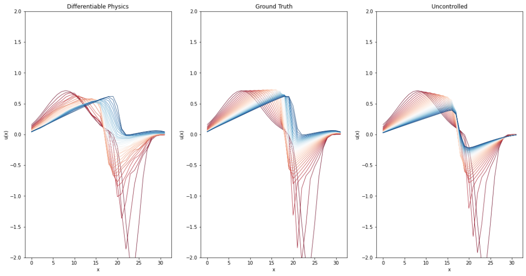
经过训练的DP模型还能够紧密地重构原始轨迹。此外,生成的结果似乎比使用RL代理更少有噪声。
因此,我们有了一个RL版本和一个DP版本,我们可以在下一节中进行更详细的比较。
16.10 RL 和 DP 的比较
接下来,通过生成的轨迹的视觉质量以及生成的力量数量进行两种方法的比较。后者提供了关于两种方法性能的见解,因为在训练过程中,两种方法都希望最小化这个度量标准。这也很重要,因为通过在最后一个时间步骤应用巨大的力量,任务可以轻松解决。因此,理想的解决方案考虑了PDE的动态,尽可能地应用少量的力量。因此,这个度量标准非常好,可以衡量网络对基础物理环境(在这个例子中是Burgers方程)的学习情况。
import utils
import pandas as pd
16.10.1 轨迹比较
为了比较结果轨迹,我们使用任一方法从测试集生成轨迹。同时,我们收集测试集场的真实模拟和自然演化。
rl_frames, gt_frames, unc_frames = rl_trainer.infer_test_set_frames()

dp_frames = dp_app.infer_all_frames(TEST_RANGE)
dp_frames = [s.burgers.velocity.data for s in dp_frames]

frames = {
    (0, 0): ('Ground Truth', gt_frames),
    (0, 1): ('Uncontrolled', unc_frames),
    (1, 0): ('Reinforcement Learning', rl_frames),
    (1, 1): ('Differentiable Physics', dp_frames),
}
TEST_SAMPLE = 0  # Specifies which sample of the test set should be displayed

def plot(axs, xy, title, field):
    axs[xy].set_ylim(-2, 2); axs[xy].set_title(title)
    axs[xy].set_xlabel('x'); axs[xy].set_ylabel('u(x)')
    label = 'Initial state (red), final state (blue)'
    for step_idx in range(0, STEP_COUNT + 1):
        color = bplt.gradient_color(step_idx, STEP_COUNT+1)
        axs[xy].plot(
            field[step_idx][TEST_SAMPLE].squeeze(), color=color, linewidth=0.8, label=label)
        label = None
    axs[xy].legend()

fig, axs = plt.subplots(2, 2, figsize=(12.8, 9.6))
for xy in frames:
    plot(axs, xy, *frames[xy])
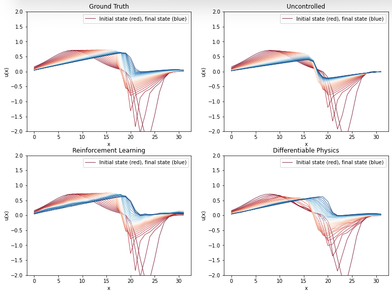
这张图将上面两个训练后的图表连接在一起。我们再次看到,可微物理方法似乎比强化学习代理生成的轨迹更少噪声,而两者都能近似地逼近真实情况。
16.10.2 生成力的比较
接下来,我们计算各个方法产生并应用于测试集轨迹的力。
gt_forces = utils.infer_forces_sum_from_frames(
    gt_frames, DOMAIN, DIFFUSION_SUBSTEPS, VISCOSITY, DT
)
dp_forces = utils.infer_forces_sum_from_frames(
    dp_frames, DOMAIN, DIFFUSION_SUBSTEPS, VISCOSITY, DT
)
rl_forces = rl_trainer.infer_test_set_forces()
Sanity check - maximum deviation from target state: 0.000000
Sanity check - maximum deviation from target state: 0.000011
首先,我们将比较RL和DP方法生成的力的总和,并将其与实际情况进行比较。
plt.figure(figsize=(8, 6))
plt.bar(
    ["Reinforcement Learning", "Differentiable Physics", "Ground Truth"],
    [np.sum(rl_forces), np.sum(dp_forces), np.sum(gt_forces)],
    color = ["#0065bd", "#e37222", "#a2ad00"],
    align='center', label='Absolute forces comparison' )
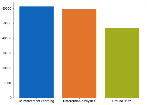
如图所示的条形图所示,DP方法学习应用的力略低于RL模型。
由于两种方法在达到最终目标状态方面表现相当,因此这是我们用来比较两种方法性能的主要数量。接下来,方法生成的力也与各样本的真实情况进行了视觉比较。放置在蓝线上方的点表示分析的深度学习方法比地面实况产生更强的力,反之亦然。
plt.figure(figsize=(12, 9))
plt.scatter(gt_forces, rl_forces, color="#0065bd", label='RL')
plt.scatter(gt_forces, dp_forces, color="#e37222", label='DP')
plt.plot([x * 100 for x in range(15)], [x * 100 for x in range(15)], color="#a2ad00", label='Same forces as original')
plt.xlabel('ground truth'); plt.ylabel('reconstruction')
plt.xlim(0, 1200); plt.ylim(0, 1200); plt.grid(); plt.legend()
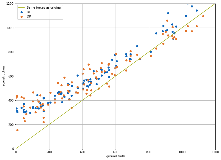
图表显示,DP训练运行的橙色点通常更接近对角线 - 即,该网络学会了生成更接近真实值的力。
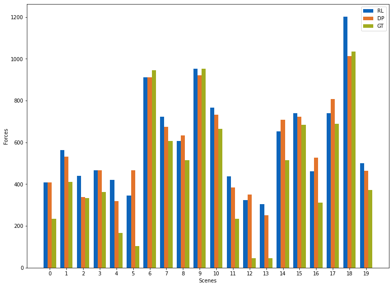
下图显示了所有强化学习、可微分物理和基准真值在个体样本上的表现。
w=0.25; plot_count=20   # How many scenes to show
plt.figure(figsize=(12.8, 9.6))
plt.bar( [i - w for i in range(plot_count)], rl_forces[:plot_count], color="#0065bd", width=w, align='center', label='RL' )
plt.bar( [i     for i in range(plot_count)], dp_forces[:plot_count], color="#e37222", width=w, align='center', label='DP' )
plt.bar( [i + w for i in range(plot_count)], gt_forces[:plot_count], color="#a2ad00", width=w, align='center', label='GT' )
plt.xlabel('Scenes'); plt.xticks(range(plot_count))
plt.ylabel('Forces'); plt.legend(); plt.show()
16.11 训练进度比较
虽然以上设置的主要目标是力量大小方面的控制质量,但在训练时,两种方法的行为方式存在有趣的差异。物理无感知的强化学习训练和具有紧密耦合求解器的DP方法的主要差异在于后者的收敛速度明显更快。即,数值求解器提供的梯度比RL过程的无指导探索提供更好的学习信号。另一方面,RL训练的行为部分可以归因于训练数据收集的策略性和强化学习技术的“蛮力”探索。
下一个单元格将可视化两种方法在墙时方面的训练进展。
def get_dp_val_set_forces(experiment_path):
    path = os.path.join(experiment_path, 'val_forces.csv')
    table = pd.read_csv(path)
    return list(table['time']), list(table['epoch']), list(table['forces'])

rl_w_times, rl_step_nums, rl_val_forces = rl_trainer.get_val_set_forces_data()
dp_w_times, dp_epochs, dp_val_forces = get_dp_val_set_forces(DP_STORE_PATH)

plt.figure(figsize=(12, 5))
plt.plot(np.array(rl_w_times) / 3600, rl_val_forces, color="#0065bd", label='RL')
plt.plot(np.array(dp_w_times) / 3600, dp_val_forces, color="#e37222", label='DP')
plt.xlabel('Wall time (hours)'); plt.ylabel('Forces')
plt.ylim(0, 1500); plt.grid(); plt.legend()
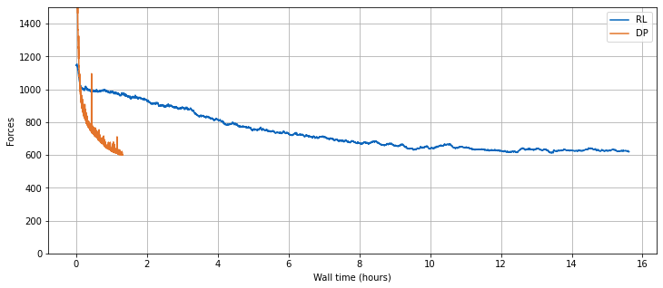
综上所述,与可微分物理方法相比,PPO强化学习施加的力更高。因此,PPO得到的学习解决方案质量略微劣。此外,在强化学习情况下,收敛所需的时间显著更长(无论是在墙上的时间还是在训练迭代中)。
16.12 下一步
- 观察超参数(如学习率)不同取值对训练过程的影响
- 使用不同分辨率的场,并比较两种方法的差异。更高的分辨率会使物理动力学更加复杂,因此更难控制
- 在不同环境参数(如粘度、dt)的设置中使用训练好的模型,并测试它们的泛化能力